0%

深度学习系列第六篇 — 卷基层和池化层展示

练习代码

1
2
3
4
5
6
7
8
9
10
11
12
13
14
15
16
17
18
19
20
21
22
23
24
25
26
27
28
29
30
31
32
33
34
35
36
37
38
39
40
41
42
# -*- coding:utf-8 -*-
import tensorflow as tf
from tensorflow.examples.tutorials.mnist import input_data
import matplotlib.pyplot as plt
import matplotlib.gridspec as gridspec
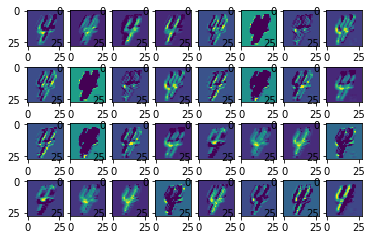
# 下载或加载数据
mnist = input_data.read_data_sets("MNIST_data", one_hot=True)


def weight_variable(shape):
inital = tf.truncated_normal(shape, stddev=0.1)
return tf.Variable(inital)


def bias_variable(shape):
inital = tf.constant(0.1, shape=shape)
return tf.Variable(inital)


def conv2d(x, w):
return tf.nn.conv2d(x, w, strides=[1, 1, 1, 1], padding='SAME')


def max_pool_2x2(x):
return tf.nn.max_pool(x, ksize=[1, 2, 2, 1], strides=[1, 2, 2, 1], padding='SAME')


xs = tf.placeholder(tf.float32, [None, 784]) # 28 * 28
ys = tf.placeholder(tf.float32, [None, 10])
x_image = tf.reshape(xs, [-1, 28, 28, 1])
# conv1 layer #
w_conv1 = weight_variable([5, 5, 1, 32]) # patch 5 x 5, in size 1, out size 32
b_conv1 = bias_variable([32])
h_conv1 = tf.nn.relu(conv2d(x_image, w_conv1) + b_conv1) # output size 28 x 28 x 32
h_pool1 = max_pool_2x2(h_conv1) # output size 14 x 14 x 32

# conv2 layer #
w_conv2 = weight_variable([5, 5, 32, 64]) # patch 5 x 5, in size 32, out size 64
b_conv2 = bias_variable([64])
h_conv2 = tf.nn.relu(conv2d(h_pool1, w_conv2) + b_conv2) # output size 14 x 14 x 64
h_pool2 = max_pool_2x2(h_conv2) # output size 7 x 7 x 64
Extracting MNIST_data/train-images-idx3-ubyte.gz
Extracting MNIST_data/train-labels-idx1-ubyte.gz
Extracting MNIST_data/t10k-images-idx3-ubyte.gz
Extracting MNIST_data/t10k-labels-idx1-ubyte.gz

输出结果

两层卷基层和两层池化层的处理结果展示出提取出的图像特征

1
2
3
4
5
6
7
8
9
10
11
12
13
14
15
16
17
18
19
20
21
22
23
24
25
26
27
28
29
30
31
32
33
34
35
36
37
38
39
40
41
42
43
44
45
46
47
48
49
50
with tf.Session() as sess:
sess.run(tf.global_variables_initializer())
batch_xs, batch_ys = mnist.train.next_batch(1)

h_conv1_res, h_pool1_res, h_conv2_res, h_pool2_res = \
sess.run([h_conv1, h_pool1, h_conv2, h_pool2],
feed_dict={xs: batch_xs, ys: batch_ys})

input_x = batch_xs.reshape([28, 28])
print "Show input:"
print "input shape:", input_x.shape
gs1 = gridspec.GridSpec(1, 1)
plt.imshow(input_x)
plt.show()

print "Show first conv2d result:"
print "conv2d shape:", h_conv1_res.shape
gs1 = gridspec.GridSpec(4, 8)
for x in range(4):
for y in range(8):
plt.subplot(gs1[x, y])
plt.imshow(h_conv1_res[0, :, :, x * 4 + y])
plt.show()
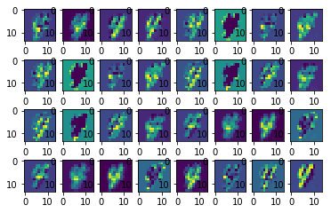
print "Show first max_pool result:"
print "max_pool shape:", h_pool1_res.shape
gs1 = gridspec.GridSpec(4, 8)
for x in range(4):
for y in range(8):
plt.subplot(gs1[x, y])
plt.imshow(h_pool1_res[0, :, :, x * 4 + y])
plt.show()
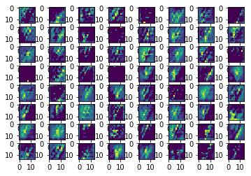
print "Show second conv2d result:"
print "conv2 shape:", h_conv2_res.shape
gs1 = gridspec.GridSpec(8, 8)
for x in range(8):
for y in range(8):
plt.subplot(gs1[x, y])
plt.imshow(h_conv2_res[0, :, :, x * 8 + y])
plt.show()
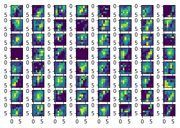
print "Show second max_pool result:"
print "max_pool shape:", h_pool2_res.shape
gs1 = gridspec.GridSpec(8, 8)
for x in range(8):
for y in range(8):
plt.subplot(gs1[x, y])
plt.imshow(h_pool2_res[0, :, :, x * 8 + y])
plt.show()
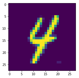
Show input:
input shape: (28, 28)

png

Show first conv2d result:
conv2d shape: (1, 28, 28, 32)

png

Show first max_pool result:
max_pool shape: (1, 14, 14, 32)

png

Show second conv2d result:
conv2 shape: (1, 14, 14, 64)

png

Show second max_pool result:
max_pool shape: (1, 7, 7, 64)

png

卷基层和池化层的处理

卷积层部分被称之为过滤器(或者内核)

单位节点矩阵指长和宽都为1,深度不限的节点矩阵。

过滤器处理的矩阵深度和当前层神经网络节点矩阵的深度一致。

过滤器的处理方式如下图:

convolution_schematic

卷基层的参数个数 = 过滤器尺寸 × 输入矩阵深度 × 卷基层深度 + 卷基层深度(偏置个数)

池化层处理可以非常有效的缩小矩阵的尺寸,同时可以防止过拟合的问题。池化层的计算通常有两种方式,一种是最大池化层,另一种是取平均值的平均池化层。

池化层处理方式:

pooling_schematic

其它工具用法总结

matplotlib 图像行内显示: %matplotlib inline

通过 PIL 加载图像:Image.open('img/cnn_sample_test.jpg')

图像转 numpy array: numpy.asarray(img, dtype='float32')

numpy array 转 PIL 图像: Image.fromarray(img[:, :, :], 'RGB')

第一个参数是 array ,第二个参数是图像的模式,灰度图像为 L,彩色图像为 RGB, 灰度图像深度为1,是一个二维矩阵,RGB图像为三层深度的二维矩阵。

PIL 多图像拼接显示:

1
2
3
4
5
6
7
8
gs1 = gridspec.GridSpec(3, 5)
for i in range(3):
plt.subplot(gs1[i, 0]); plt.axis('off'); plt.imshow(img[:, :, :])
plt.subplot(gs1[i, 1]); plt.axis('off'); plt.imshow(conv_op[0, :, :, i])
plt.subplot(gs1[i, 2]); plt.axis('off'); plt.imshow(sigmoid_op[0, :, :, i])
plt.subplot(gs1[i, 3]); plt.axis('off'); plt.imshow(avg_pool_op[0, :, :, i])
plt.subplot(gs1[i, 4]); plt.axis('off'); plt.imshow(max_pool_op[0, :, :, i])
plt.show()

gridspec.GridSpec(3, 5) 可以理解为将一个画布分成 3 × 5 的方格

plt.subplot(gs1[0, 0]); plt.axis('off'); plt.imshow(img[:, :]) 选择第一个画布,将图像填充到这个画布下,并且不显示坐标。

参考资料:

http://mourafiq.com/2016/08/10/playing-with-convolutions-in-tensorflow.html

欢迎关注我的其它发布渠道